Towards Solving Connect Four 3D
Introduction
Connect Four 3D (aka Sogo, Connect Four advanced, or Score Four) is a two player strategy game. It is a three-dimensional version of the game Connect Four and is played on a three-dimensional 4x4x4 board. Both players alternate to place their stones in one of the columns unless it already contains four stones. The stone then falls to the bottom of the column. The player who manages first to position four stones in a straight line on any level or angle wins the game. Connect Four is very similar to 3D Tic Tac Toe (aka Qubic), with the difference that Qubic is without "gravity", which means that stones can be placet at any free spot. While Patashnik proved that Qubic is a first player win already in 1980[8], Connect Four 3D is still unsolved.
The goal of this project is to progress towards solving Connect Four 3D. Particularly, the goal was to improve the solver developed in the thesis of Deutrich[3], who adapted many ideas presented in the excellent blog about solving Connect Four of Pascal Pons [5]. In the current project, I present two solvers: The first one is an implementation of the Minimax algorithm with improved heuristics that attempts to solve a position as fast as possible on a single CPU. The second solver distributes the search among many Minimax solvers of the first kind to achieve much better performance by using parallelism.
The solvers presented here are implemented using C++. For parallelism we use the OpenMP library[6]. The parallel solver runs on the CooLMUC-2 cluster which is part of the Linux cluster of the LRZ[7].
Minimax Solver
The minimax solver implements the recursive minimax algorithm to solve Connect Four 3D positions. In this chapter the bitboard, move order and transposition table are presented. Instead of using alpha-beta pruning, we make the additional assumption that connect four 3D is a first player win, and prune the search tree as follows: When the second player finds a draw, his other possible moves are pruned, since this is the best he can achive. If the search returns a first player win, then he can force a win from that position. In particular, there's no distinction between a draw and a second player win. A similar technique was used for the checkers solver Chinook [9].
Next, we introduce some abbreviations for some important recurring patterns. If a player has three stones in a line, the empty fourth position is called a threat. If the player can play the thread and win the position, it is called an opening. If a player can move while having an opening that player wins the game. By anticipating bad moves, the number of explored nodes can be decreased. In particular, the following situations can be efficiently detected by using a bitboard implementation.
- The player has an opening.
- The opponent has one opening.
- The opponent has two openings.
- the opponent has a threat above the opening of the current player.
- The second player has a stone in every line.
- The first player doesn't win by placing the 63th stone.
These positions yield either to a forced move or to a decisive move and do not require further exploration.
Bitboard
A bitboard is an encoding of a position into a bitmap. Representing the game board as bitboard allows us to manipulate it efficiently using bitwise operations. They are essential to increase the performance of the solver. The bitboard presented here is the same Deutrich[3] used, which in turn is based on a bitboard by Pons[5] for connect four. The idea is to map the stones of each player to a 64 bit integer. The following table shows how the positions of the game board are mapped to the 64 bit integer. The lowest bits 0 to 15 encode the first layer of the game board, the next 16 bits the second layer and so fort.
48 49 50 51
52 53 54 55
56 57 58 59
60 61 62 63

32 33 34 35
36 37 38 39
40 41 42 43
44 45 46 47

16 17 18 19
20 21 22 23
24 25 26 27
28 29 30 31

0  1  2  3
4  5  6  7
8  9 10 11
12 13 14 15
For each player then a bit is set to 1 if the player has a stone at that position, otherwise the bit is set to 0. The number of stones placed in total and the locations of threats for each player are also saved in the bitboard so that they do not need to be computed each time. A different variant that stores the whole board in only 80 bits is used to store a position in the transposition table.
Move Order
The move order used for the minimax solver is based on a heuristic that assigns each move a score based on the other stones that are connected to the move. For each line that contains a stone of the other player no points are awarded. The point values can be seen in the following table.
| Stones of player | Score |
|---|---|
| Any | 0 |
| 0 | 1 |
| 1 | 10 |
| 2 | 100 |
| Opening created | 1000 |
Notice how lines where stones of the opponent are placed give no points. Each player focuses on improving his own position and not on making the opponent worse off. Creating an opening gives a bigger score than a threat that has no direct consequences. Since each stone is part of at most 7 lines the scores of one level can never surpass the next higher ones. So if a move is the first stone in seven lines it gets a score of 7. It is considered worse than a move that is the second stone in one line and gets no points in all others, with a score of 10. The moves are ordered using insertionsort from best to worst.
The order in which the possible moves of a player are searched by the minmax solver has a big impact on the performance of the algorithm. For example, if all choices for the max player are wins, then the choice doesn't matter. But if some moves lead to a loss, moves need to be explored until one winning move is found. If all moves are a loss then all need to be explored. It is therefore important to order moves such that the best moves are explored first. Despite putting in a lot of effort and testing, improving the move oreder turned out to be particularly hard. The current move ordering performs quite well for the middle- and endgame (>25 stones), but there is certainly room to improve when there are less stones. However, exhaustively testing different heuristics is almost impossible for positions with few stones.
Transposition Table
In Connect Four 3D, like in many other games like chess, one position can be reached by different lines of play. As a result the game tree contains many duplicate nodes or should be seen as a directed acyclic graph (DAG). Saving all visited nodes during search requires too much memory. The transposition table is a solution to this problem. It is a fixed size table that saves positions and their solutions. New positions can then be searched in the transposition table to check if they are already solved and the fixed size allows it to fit into memory. It is implemented as a fixed size hash table to allow for constant time insert and find operations. The following points need to be addressed when using a transposition table:
Symmetries of the same game board should be mapped to the same entries.
Minimizing the entry size to increase the number of stored positions.
Hash function, maps positions to table entries.
Replacement strategy, decides which positions to replace when the table is full.
Thread safety, to allow multiple threads to work on the same transposition table.
Thread safety is only required if multiple threads are sharing the transposition table, otherwise it will only be an overhead.
Symmetries
Connect Four 3D has 8 symmetries. All 8 different boards can be computed by flipping each layer horizontally, vertically or diagonally. When inserting or searching for a board, all 8 symmetric boards are computed. The one with the lowest numerical value is then chosen as the canonical key that represents all 8 boards. Here are the three flip functions that perform the left right (LR), up down (UD) and diagonal (DI) flips. They use masks to select a part of the board, move it with shifts and then recombine the moved parts. The function that computes the canonical key uses these three functions to compute the 8 symmetries of a position and then chooses the minimum.
inline uint64_t Board::flipLR(uint64_t b) {
    return  ((b & 0x8888888888888888) >> 3) |
            ((b & 0x4444444444444444) >> 1) |
            ((b & 0x2222222222222222) << 1) |
            ((b & 0x1111111111111111) << 3);
}

inline uint64_t Board::flipUD(uint64_t b) {
    return  ((b & 0xF000F000F000F000) >> 12) |
            ((b & 0x0F000F000F000F00) >>  4) |
            ((b & 0x00F000F000F000F0) <<  4) |
            ((b & 0x000F000F000F000F) << 12);
}

inline uint64_t Board::flipDI(uint64_t b) {
    return  ((b & 0x8000800080008000) >> 15) |
            ((b & 0x4800480048004800) >> 10) |
            ((b & 0x2480248024802480) >>  5) |
             (b & 0x1248124812481248)        |
            ((b & 0x0124012401240124) <<  5) |
            ((b & 0x0012001200120012) << 10) |
            ((b & 0x0001000100010001) << 15);
}
Reducing the Transposition Table Entry Size
The naive transposition table entry saves the bitboard, the outcome and any other information needed by the replacement strategy. The outcome is 1 bit of information, first player wins or does not win. The space needed by the replacement strategy depends on which one is chosen and may vary from 0 bit to multiple bytes. The space needed by the bitboard used for computations would be 128 bit. This can be reduced to 32 bits (and potentially less) by first mapping the bitboard to a compact representation and then only saving the last $k$ bit.
Compact bitboard
The compact bitboard stores the same information as the regular bitboard in only 80 bit. The idea is to represent stones of the first and second player by a 1 and 0 respectively. Then the first empty position in each column is indicated by a 1 and all positions above are a 0. This representation needs 80 bits since the full board has 64 placed stones and 16 indicators on top of each column. In the following code b and ob contain the board of the first and second player respectively. At the end the variable cover contains the 16 most significant bits and the variable board the other 64 bits of the compact encoding. The idea of the code is to find the lowest empty spots, i.e., the first empty place in each column and mark it with a 1. Then that variable can be added to the board of the first player and the compact board is found.
// 1 for all filled positions
uint64_t filled = b | ob;
// Highest layer is 1 iff the column is full.
uint64_t cover = filled >> 48;
// 1 for all empty positions
uint64_t empty = ~filled;
// Lowest empty spot is empty and has no empty spot under it
uint64_t lowestEmptySpot = empty ^ (empty << 16);
// The board of the current player together with the lowest empty spot give the encoding
uint64_t board = b | lowestEmptySpot;
Saving only $k$ bit of the Key
Instead of saving the full 80 bit of the compact board in the transposition table the Chinese remainder theorem can be used to save only the last $k$ bits instead. Assume the transposition table size is a large prime number $S$. The hash function is the board modulo the size $S$. Saving only the last $k$ bits of the board is equal to saving the board modulo $2^k$. The Chinese remainder theorem guarantees that the pair $(b \mod S, b \mod 2^k)$ maps to exactly one number $b \mod (S * 2^k)$. Choosing $S * 2^k > 2^{80}$, we guarantee that each pair maps to a distinct board since the modulo operation is an identity function in that value range. This property prevents collisions in the trasposition table, since two different boards that are hashed to the same transposition table entry must be different in their last k bits. The other way also holds that if two positions have the same last k bits their hash values are different. The transposition table used when running the parallel solver on the cluster used $S = 2813000011$ entries. This number is a prime and larger than $2^{31}$. So by now choosing $k = 49$ the constraint $S * 2^{49} > 2^{31} * 2^{49} = 2^{80}$ is fulfilled. Only the last 49 bit of the compact board need to be saved in the transposition table. If we add 1 bit for the result 14 bit of the 64 bit integer remain empty. These can be used to store other helpful information.
Hash Function
The hash function is the canonical key $k$ modulo $S$, where $S$ is the size of the transposition table and a prime number. The compact representation has a size of 80 bit, so the modulo operation does not fit into one operation on a 64 bit machine. Rewrite the key as $k = a * 2^{64} + b$ where $a$ are the 16 most significant bits and b are the other 64 bits. Then the following are equivalent.
$$ a * 2^{64} + b \mod S $$$$ a * 2^{48} * 2^{16} + b \mod S $$$$ (a * 2^{48} \mod S) * 2^{16} + (b \mod S) \mod S $$Observe that in the third row all numbers and intermediate results fit into 64 bit. No overflow can happen as long as $S < 2^{48}$. From second to third step, we used the fact that the result does not change if we insert additional modulo S operations.
hash = (cover << 48)  % TranspositionTable::SIZE;
hash = ((hash  << 16) + (board % TranspositionTable::SIZE)) % TranspositionTable::SIZE;
The multiplications with powers of 2 is implemented as shifts. This implementation performs 3 modulo operations. The cover are the 16 most significant bits of the key in a 64 bit integer and the board are the other 64 bits.
Replacement Strategy for the transposition table
We save evaluated positions in the transposition table with the idea to avoid repeated calculation. The transposition table is implemented as a hash table. The insert operation can result in collisions, and in fact the table will be filled after a short while and every insert operation will result in a collision. When that happens, a decision has to be made about which position to keep and which one to discard. These decisions are the replacement strategy. For a discussion of replacement strategies see [2]. The most interesting replacement strategies, from the paper are:
- NEW always replace the old entry with the new.
- BIG compare the subtree size of the entries and keep the one with the larger subtree
- TWOBIG combination of NEW and BIG. Each entry can hold 2 positions. A new entry is first compared with the first position and the one with the larger subtree gets the spot, like in BIG. The other one replaces the second entry, like in NEW.
NEW is good since it always saves new positions. This is desirable since positions that were visited recently have a high chance to be seen again. This happens when one position is reached by lines of play that are just permutations of each other. Very expensive positions may get overwritten by the time they are seen again. BIG solves this problem by always keeping the most expensive position in terms of how long it took to solve. However, small positions are never saved into the transposition table by this approach. While finding them only saves little time they are also the ones most frequently found. TWOBIG is a compromise between the two. It gives half of the transposition table to the largest and the other half to new entries.
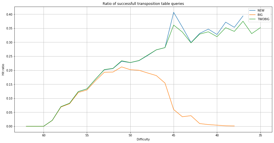
The quality of a replacement strategy is given by two properties. The first one is the hit ratio. Each time a position that was already solved is found in the transposition table time is saved, but not each hit saves the same amount of time. Generally, the larger the subtree, the more time is saved when a hit occurs. The following figure shows a direct comparison between NEW, BIG and TWOBIG. Overall the hit ratio is maximal for NEW. We see that BIG quickly runs into the problem that the whole transposition table gets filled with difficult positions and that the hit ratio quickly goes to zero since the majority of the solved positions will always be at the lowest levels. The TWOBIG strategy performs the best. While it has a slightly lower hit ratio than NEW it manages to allow the solver to solve difficulty 36 and 35 while NEW fails at 36. This means TWOBIG had a large performance impact even with a lower hit rate. Based on this result the minimax solver works with a TWOBIG replacement strategy for the transposition table.
Thread safe Transposition Table
A parallel solver distributes the work among multiple threads, which should share one transposition table to benefit from having access to positions solved by other threads. To allow this, the transposition table has to be thread-safe to prevent threads from accessing the same memory at the same time, atomic read/write operations are guaranteed to be executed completely and that no other thread executes a operation at the same time on the same value. Implementing all reads and writes from and to the transposition table as atomic operations makes the transposition table thread-safe. This only works because the entries are exactly 64 bit large. Most systems only allow for atomic operations on 64/32/16/8 bit data. This does not guarantee that no 2 threads try to insert a entry at the same position in the transposition table. It just guarantees that the reads and writes, while following the replacement strategy, are not done at the same time. This means all entries in the transposition tables and all read entries are always correct. Threads may overwrite entries of each other, so the transposition table will look different depending on the order in which the operations are executed. Completely loosing a entry is also possible. Using atomic operations is a computationally cheap method to gain thread safety, but it sacrifices the correctness of the replacement strategy. Since they are heuristics and don't change the result and only the run time, this trade off is acceptable. Below is an example of how a atomic read and write operation looks like using OpenMP directives. They look like standard C++ assignments. The #pragma omp compiler directives change them to atomic operations during compilation.
#pragma omp atomic read
uint64_t oldEntry = transpositionTable[b.hash];

#pragma omp atomic write
transpositionTable[b.hash] = newEntry;
In the previous chapters methods where shown to reduce the size of each table entry to a 64 bit integer. For TWOBIG, 2 entries are saved at each position. Each table entry needs therefore 16 bytes and contains 2 positions. The size of the transposition table is therefore $16 * S$ bytes. For the CooLMUC-2 cluster $S = 2813000011$ is chosen. This means it requires $2 * 8 * S \text{ byte} = 16 * 2813000011 \text{ byte} = 45008000176 \text{ byte} = 45.01 \text{ GB}$ of memory. CooLMUC-2 cluster nodes provide 64 GB of memory. The transposition table fits and leaves 19 GB of memory for the parallel solver to coordinate execution.
Performance Test
In this chapter, the solver is evaluated. The graphs contain a comparison for the evaluation of a modified version of the negamax solver by Deutrich[3]. The tests measure total time, time per position and the total number of evaluated positions. The tests are divided into difficulties. The difficulty is given by the number of already placed stones, e.g., a difficulty of 40 means that 40 of 64 stones are already placed and that it's the first players turn. The difficulty of 0, i.e., the empty board is the hardest position. The more stones are placed, the easier the positions are in general. The solver was tested on 1000 positions for each difficulty. These where randomly and uniformly drawn from the distribution of random legal and reasonable play sequences. This means no player is allowed to lose, i.e., a player is forced to prevent a win if possible and otherwise chooses randomly and uniformly between his legal moves. The tests were performed on a laptop pc with a Intel i5 processor. The solver had a time limit of 10 minutes to solve 1000 positions of one difficulty and a transposition table with a size of 1 gigabyte.
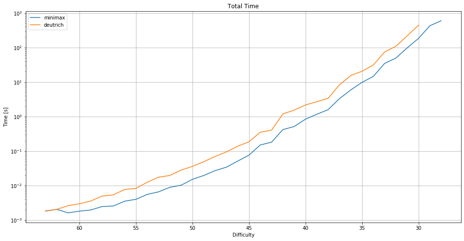
The minimax solver can solve 1000 positions with 28 stones placed in 597 seconds. This is barely below the allowed time of 600 seconds. The solver doesn't solve difficulty 27 in the given time limit. The needed time grows exponentially with the difficulty. Any time the solver spends on initialization, e.g., of the transposition table, is also counted.
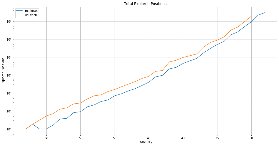
The number of explored positions also grows exponentially. The minimax solver visits 3,011,510,874 positions in 10 minutes for difficulty 28. From one difficulty to the next the number of positions that need to be visited grows by a factor between $1.2$ and $2$.
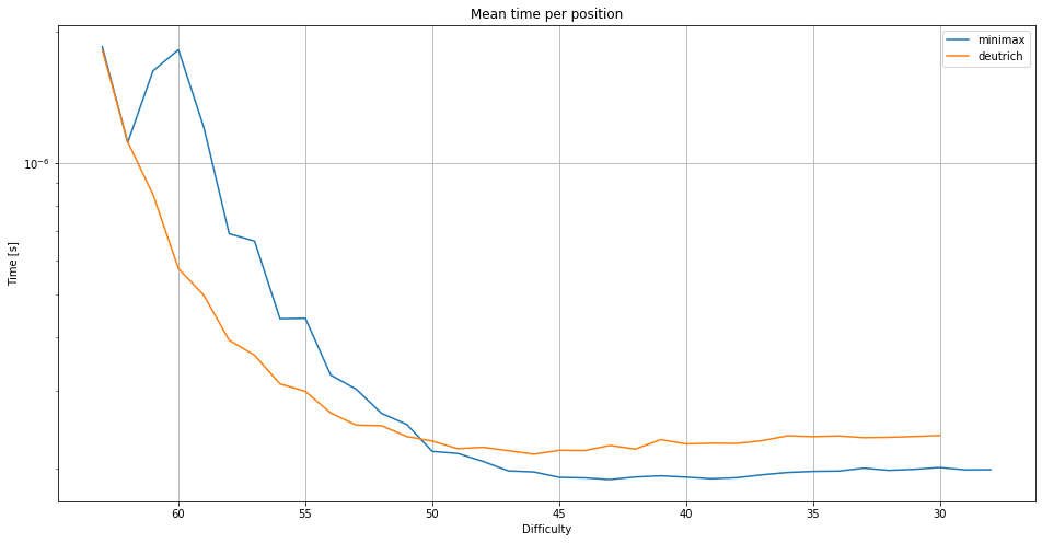
The minimax solver solves on average one position every 200 nanoseconds or 5 million positions each second.
Parallel Minimax Solver
The parallel minimax solver achieves parallelism by dividing the game tree among multiple minimax solvers that share one transposition table. Dividing the game tree to achieve a high speedup and efficiency is a very challenging problem. The speedup of a parallel implementation is the factor of how much faster it is than searching on a single core, e.g., if 4 cores can solve the problem in half the time then the speedup is 2. The efficiency is the speedup divided by the number of cores, e.g., in the previous example, the efficiency is $\frac{2}{4} = 0.5$. It expresses how much work each thread in the parallel case performs compared to the single core case. It happens frequently that the more cores one assigns to a problem the lower the efficiency becomes. This is undesirable since doubling the number of cores could then lead to only gaining a small speedup or none at all. The goal of this implementation is to achieve an efficiency of one, so that we get a linear speedup where doubling the number of cores means halving the needed time.
The parallel minimax solver is built on pseudo code for Proof Number search (PN) by Kishimoto[4]. It was then changed to search the game tree in the same order as minimax search. It builds the whole search tree up to a certain depth, to prevent solving difficult positions multiple times.
Choosing which positions to solve in parallel
In the paper Job-Level Proof-Number Search for Connect6[3], an extension to PN search was proposed that allows each tree node to be evaluated by a different heavy-weight job. These jobs can then be distributed to many cores. Instead of using PN search, our solver uses minimax search to build the game tree. In the paper, they assume that evaluating a single tree node is a heavy-weight job that requires multiple seconds. In connect four 3D, millions of nodes can be solved each second. Therefore, instead of considering solving single nodes, my solver considers whole subtrees as one task that are solved in parallel. For this a depth d is defined, on the cluster I used a depth of 22. The game tree is then built by minimax search until a node at depth d is reached. Instead of continuing the search from there, this node is now considered a task that should be solved in parallel. Now, the approach from the paper is used. This position is now considered a virtual win (or alternatively a virtual loss) and the search is continued. The search pretends virtual wins are wins (virtual losses are losses) and continues the search until the root is solved. All positions found this way can be solved in parallel by the minimax solver. If the assumption that they are a win (or loss) turns out to be true the search is correct, otherwise the error needs to be fixed. That can be done by propagating the change recursively to the parent position. As a result new positions need to be searched until the root is solved. An additional optimization is to check if solving a position contributes to solve the root. This is done by marking each node with a flag that indicates if a virtual win/loss is used to solve the node. If on each path from the leaf to the root a node lies that needs no virtual win/loss to be solved, then the leaf is not needed and can be discarded.
Managing the Game Tree
The game tree of Connect Four 3D contains many nodes that represent the same position. This means, it is better to represent it using a directed acyclic graph (DAG). There can be no cycles, because each move adds a stone. Nodes with the same position, taking into account symmetric boards, get combined. Nodes are saved in a binary tree using the canonical compact bitboard as key. Each one saves two lists, one for children and one for parents. This allows for fast find operations, insert operation and graph traversal. This data structure can keep the search tree between the position that it should solve and the cutoff depth in memory. In practice, this means it needed less than 19 GB of memory to save all positions between one depth 9 position and the cutoff depth of 22. Using a depth of 24 did exceed the available memory.
The Task Queue
The task queue is a thread-safe priority queue. Nodes at the depth of the cutoff are marked by virtual wins and added to the task queue. Worker threads get nodes from the task queue and solve them using the minimax solver. If the win assumption was wrong, the thread corrects the search tree and adds new tasks until the root is solved again. Then, the thread gets the next task from the queue. A priority queue is ordered by when a node is created by the minimax search. The node created first is returned first. For this, it is not the time the node is added to the task queue that counts, but the order in which the nodes where created when building the DAG. This can be done by assigning each node an increasing identification number (ID). Then, the task queue always returns the task with the smallest ID. This is important, because if a node turns out to be a loss, one of his siblings should be attempted next. The sibling is created right after the solved node so it has a small ID, but it gets added to the task queue only after the virtual win of the node was found wrong.
Problems
Here is a discussion of problems and how I solved them manually.
Threads cannot contribute to the search if the task queue is empty. This usually happens towards the end of the search. When the depth of the static tree is too small, there are not enough nodes created and distributed. Then, only a handfull of threads are working. If I noticed that the task queue is empty and only some threads regularly post solutions of positions they solved, I halted the search and continued with an increased cutoff depth.
Hyper threading degraded the performance of the solver. This feature of Intel processors allows multiple threads to run on virtual cores and share one real core. In the real core, some but not all parts are duplicated to allow many programs to perform as if they had access to more physical cores. I tried to run four solvers on the four hyper threads. The result was that each one solved less that one fourth of the positions a single solver could solve on one core. The problem is that for each solved position a context switch is performed. Resulting in an overhead of millions of context switches per second. I solved the problem by not using the feature and only creating one thread for each physical core.
The code is not portable. Especially the memory consumption needs to be carefully balanced. The transposition table size needs to be set as large as possible while leaving enough space for the DAG created by the parallel solver. I did this by hand when moving from a laptop to the CoolMUC 2 cluster. Moving from a laptop to a cluster also required a compiler change to the Intel c++ compiler (icpc).
Results
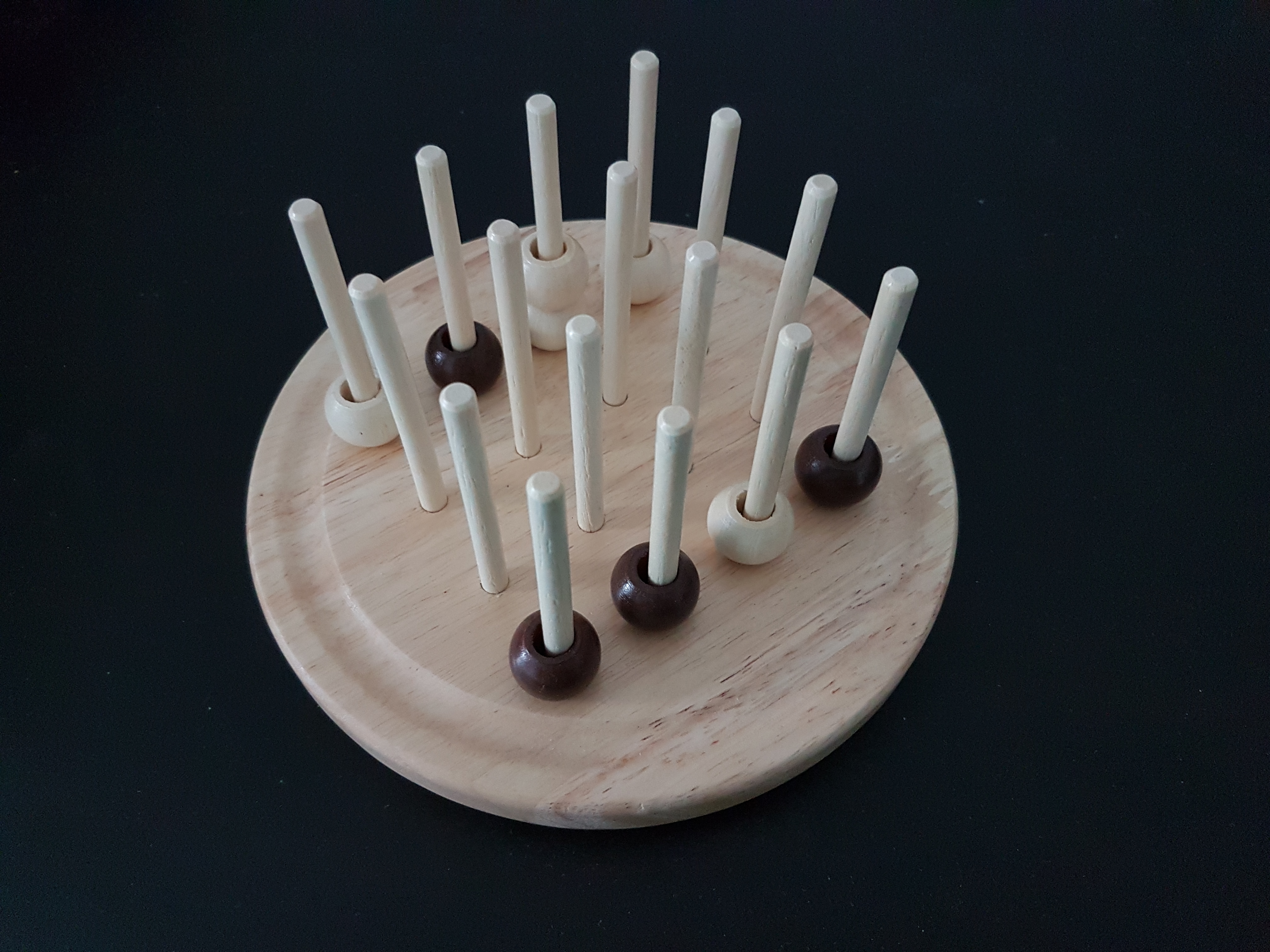
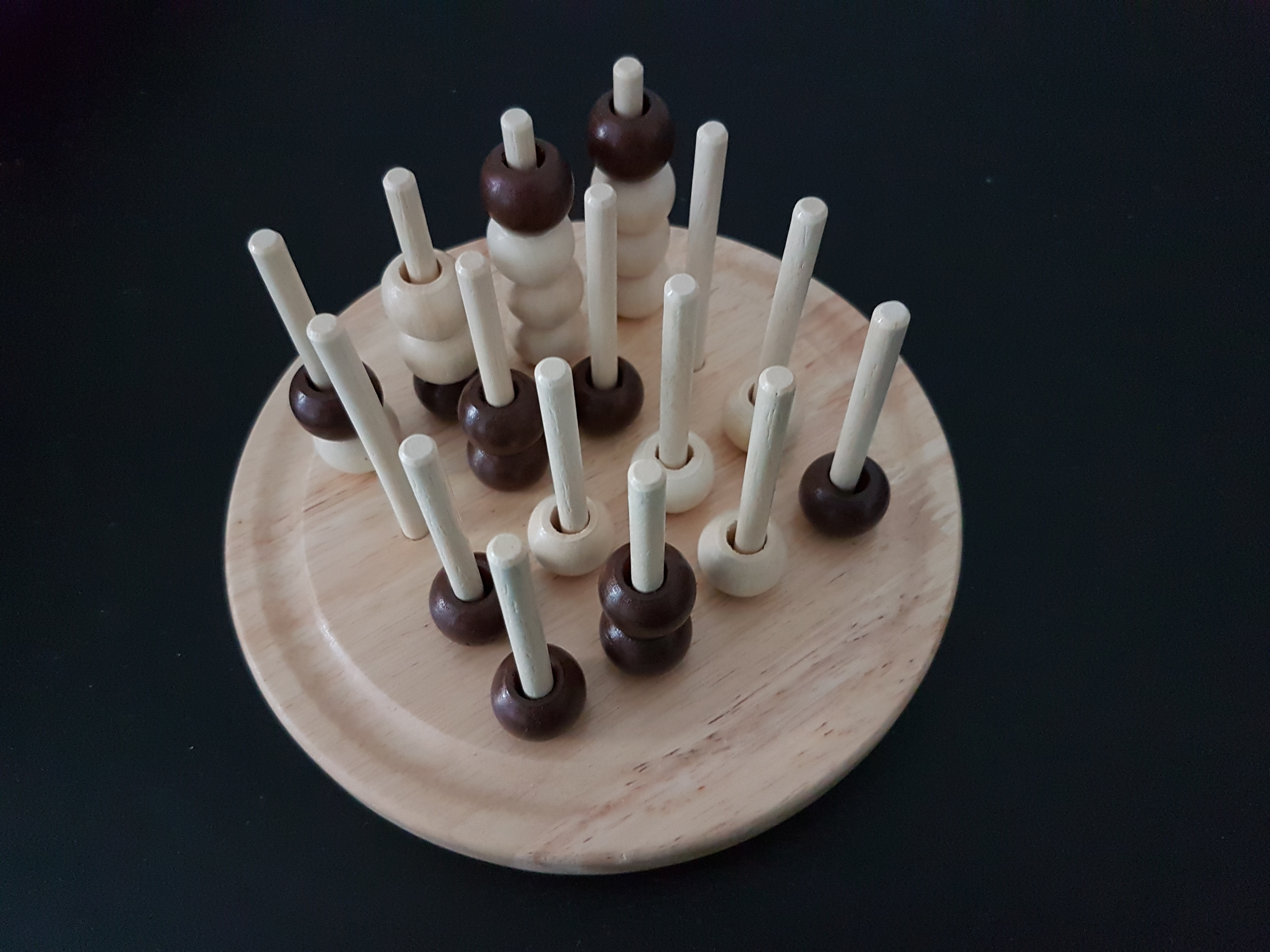
The parallel minimax solver was used to solve the position shown in the figure on the CooLMUC-2 cluster which is part of the Linux cluster of the LRZ[7]. Only 9 stones, 5 from white (first player) and 4 from black (second player) are placed. One possible sequence of moves that results in this position is the following:
| W | B | Description |
|---|---|---|
| 0 | F | White and black pick opposite corners. |
| C | 3 | White and black pick the remaining corners. |
| 4 | 8 | White picks a position between his corners, black is forced to answer. |
| 4 | B | White picks the same column again. Black picks a position between his corners. |
| 7 | White is forced to answer. Black has now 16 possible moves. |
What makes this position interesting is that almost all moves are either forced or considered to be optimal according to experienced human players. Clearly, the first moves seem very reasonable since the corners are part of 7 possible winning sets, while all other moves on the first layer are only part of 4 possible winning lines. After all corners are picked, the move by white was chosen to force black. This way, if I prove that white's next move wins after his 4th move, I have also shown that white already won after black played his second move. This means solving a position with seven stones is sufficient to solve a position with four stones in this case. To solve the position with seven stones, all 16 moves possible for black need to result in a win for white. Proving this turned out to not be feasible. Instead, I assumed that black plays B and white is forced to answer. The resulting position is the one I attempted to solve. Again all 16 possible moves for black need to be solved and result in a victory for white.
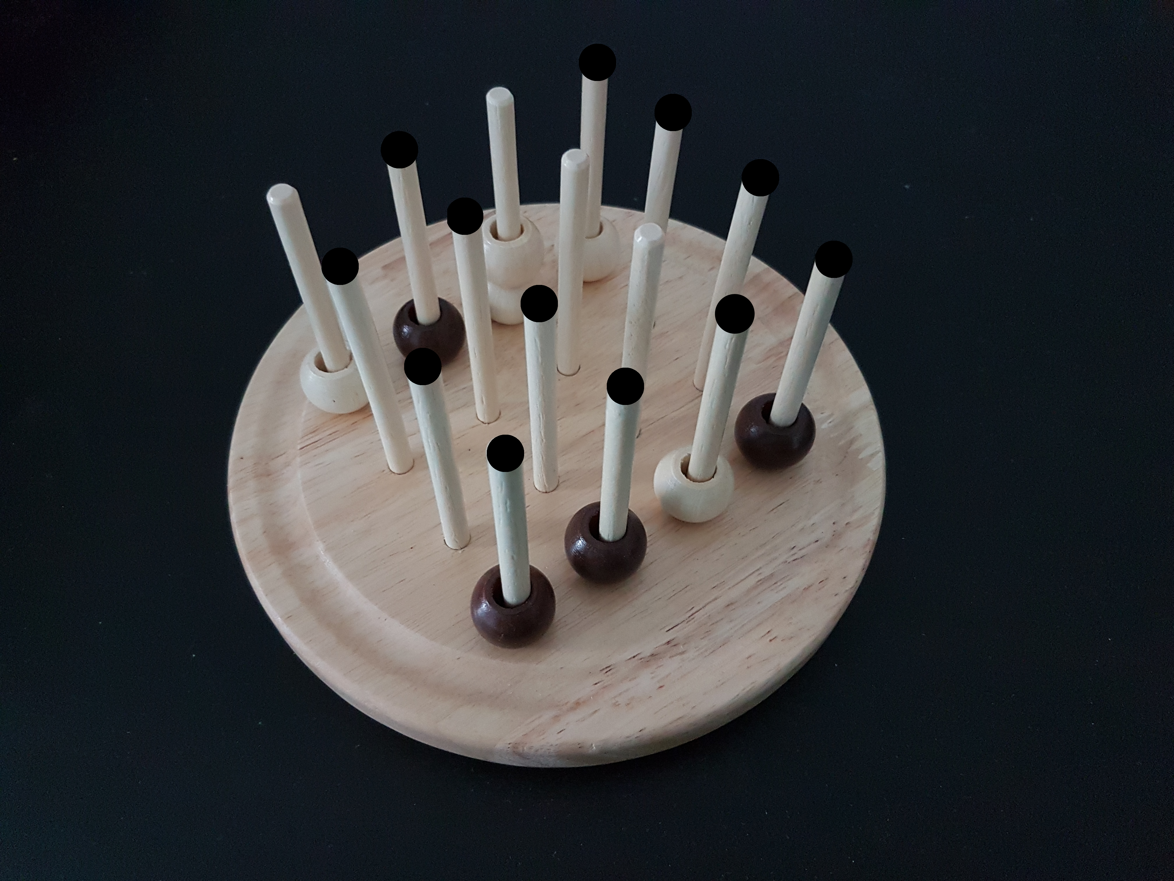
The CoolMUC 2 cluster has 28 cores per node. My solver ran on one node for over a month. In 43 days the solver explored approximately $410,000,000,000,000 = 4.1 * 10^{14}$ (410 trillion) positions. That is ca. 9.5 trillion positions explored each day, 340 billion position explored each day per core and 4 million positions each second per core. Despite all this the position above remains still unsolved. The solver showed that 12 of the 16 possible moves for black lead to a win for white. The result of the other 4 moves remain unknown. If black plays a column that is marked by a black dot, then white wins the game.
Outlook
The parallel minimax solver is capable of solving positions with 10 placed stones on a 28 core cluster. Solving the game at this speed would take years. Still, searching the game tree in parallel seems to be working well, i.e., working with multiple cpu cores, significantly imroved the performance of our solver. There are several ideas for future work.
Improving the minimax solver. While I think that it is not possible to try to explore much more than 4 million positions per second, the number of positions that need to be explored can still be reduced. For this, I think the best candidates are the move order for the early game and the transposition table.
The move heuristic was tested with 28 or more stones placed. It seems like the move order gets worse the less stones are placed. A better heuristic for positions with 10 to 28 stones could reduce the number of positions that need to be searched.
A more dynamic transposition table. The transposition table has the problem that it prefers positions with a certain number of stones. The less stones a position has, the more likely it is to receive a fixed position in the table. Most positions have many stones and they overwrite other positions in the transposition table, only positions with large subtrees are saved from this. I think that in between there are many positions that have large subtrees, but not large enough subtrees, that get overwritten by relatively unimportant positions. One idea to solve this problem is to split the transposition table into multiple tables. One for each amount of stones. All positions with 35 stones placed are then written in one transposition table and do not need to compete for space with positions that have 24 or 60 placed stones. The individual tables would be smaller, but they could also be adjusted independently. Not only their size but also the replacement strategy could be different for each depth, e.g,. the transposition table that saves positions with 60 stones could probably use NEW as replacement strategy and be relatively small. When so many stones are placed most hits are from recently seen positions and they save only little time.
References
[1] I.-C. Wu, H.-H. Lin, P.-H. Lin, D.-J. Sun, Y.-C. Chan, and B.-T. Chen. Job-level proofnumber search for connect6. In Proceedings of the 7th International Conference on Computers and Games, volume 6515, pages 11–22. Springer-Verlag, 2010.
[2] Breuker, Dennis M., Jos WHM Uiterwijk, and H. Jaap van den Herik. Replacement schemes for transposition tables. In ICGA Journal 17.4, pages 183-193, 1994.
[3] M. Deutrich. Determining the value of connect four 3d. Bachelor’s thesis, Technische Universität München, 2019.
[4] A. Kishimoto, M. H. M. Winands, M. Müller, and J.-T. Saito. Game-tree search using proof numbers: The first twenty years.International Computer Games Association Journal, 35(3):131–156, 2012.
[5] Solving Connect 4: How to build a perfect AI, Pascal Pons, https://blog.gamesolver.org/solving-connect-four/01-introduction/
[6] OpenMP, https://www.openmp.org/
[7] Leibniz-Rechenzentrum, https://www.lrz.de/
[8] Patashnik, Oren. "Qubic: 4× 4× 4 tic-tac-toe." Mathematics Magazine 53.4 (1980): 202-216.
[9] J. Schaeffer, R. Lake, Solving the game of checkers, in: R.J. Nowakowski (Ed.), Games of No Chance, MSRI Publications, Vol. 29, Cambridge University Press, Cambridge, MA, 1996, pp. 119-133.